Modelling NACA 4 digit aerofoil from equations (in creo)

Hello,

This post will cover the conception stage of aerofoil profiles and how to improve the CAD workflow for large scale simulations where multiple geometries need to be created and assessed.

One thing I have noticed is that aerofoil CAD geometry is typically produced from generating a curve through points. I have always found this cumbersome as you have to go online (typically airfoiltools.com) find the aerfoil shape that you want, download the .csv file and import it into your CAD package (with Creo you have to import .pts which requires further work and the points need to be put into a notepad file).

However, aerofoil geometries are construcuted from equations, so why not create a curve from an equation? You can set the control paramters of the design and be free to manipulate the geometry which will save you from going online to find the various profiles that you want to test.

The Equations

The NACA 4 digit profile is goverend by three distinct parameters (thickness, maximum camber, camber pos along chord) that are used in multiple equations to generate the profile.

The first equation utilises the thickness (using h instead of t as Creo reserves t for time) where 0<h. The quadratic equation can be used to plot a symmetrical aerofoil profile as it doesn't include camber parameters.

You can modify the last coefficient to -0.1036, this will result in a closed geometry.

Yt=5h[0.2969(√x)-0.126x-0.3516(x^2)+0.2843(x^3)-0.1015(x^4)]

However for cambered geometry the process is slighlty more complex. Two equations are needed to generate the mean camber line. 'm' being the maximum camber and 'p' being the position of maximum camber along the chord.

You can see that the two equations are generated from either side of the maximum camber point and therefor intersect at this location.

Yc=(m/p^2)(2px-x^2), 0<=x<=p

Yc=(1/(1-p^2))((1-2p)+2px-x^2), p<=x<=1

Applying the thickness equation Yt together with the mean camber line equation Yc you can plot the profile which is perpendicular to the camber line.

Yu=Yc+Ytcosθ

Yl=Yc-Ytcosθ

where θ=arctan(dYc/dx) 

and

dYc/dx=(m/p^2)(p-x), 0<=x<=p

dYc/dx=(m/(1-p^2))(p-x), p<=x<=1

Curve Generation

Within Creo model properties it is important to set the length unit to base unit meter (or inch if your imperial). This is becasuse chord length isn't a parameter setup in the governing equations, therefor a chord length of 1mm would be too small.

figure 1 - Model properties

Within the parameters window the 3 goverining paramtes can be setup. Figure 2 shows that it is currently set to thickness of 12%, maximum camber of 2% and positon at 40% of the chord length giving an aerofoil designation of 'NACA 2412' .

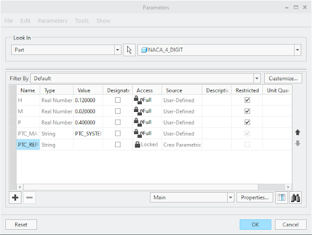figure 2 - Parameters window settings

With the parameters set, the curves can be genertated. I have found that with the curve through equation tool you can't create a relation between a parameter and the x limit so you have to create 4 seperate curves (2 for the upper surface and 2 for the lower surface).

In figure 3 the cuve for the equation is projected and figure 4 shows the equation required to generate it.

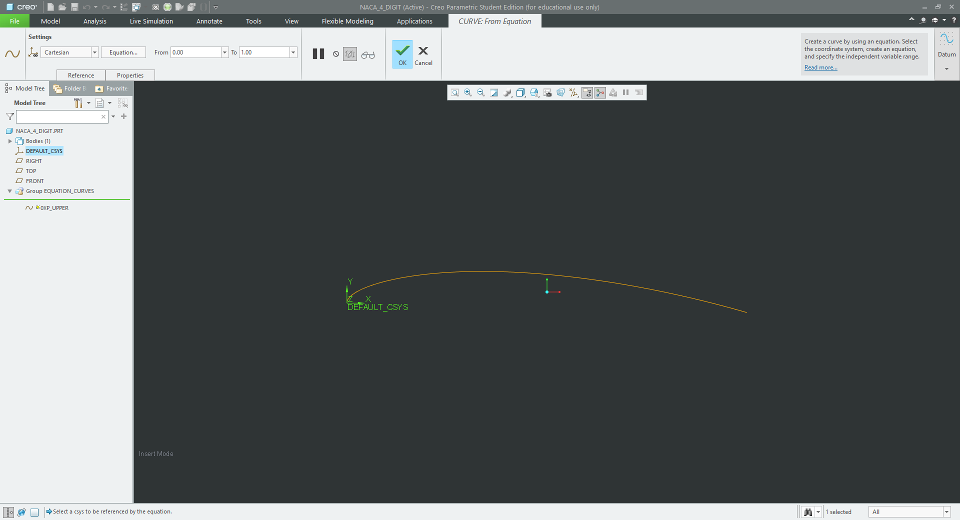figure 3 - curve from equation of upper surface 0<=x<=P

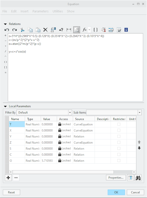figure 4 - equation for curve upper surface 0<=x<=P

This process is repeated a further three times until you end up with 4 curves as seen in figure 5. I have also created a sketch which includes a point and axis which is related to the paramter 'p' this will help with the future steps for generating the surfaces.

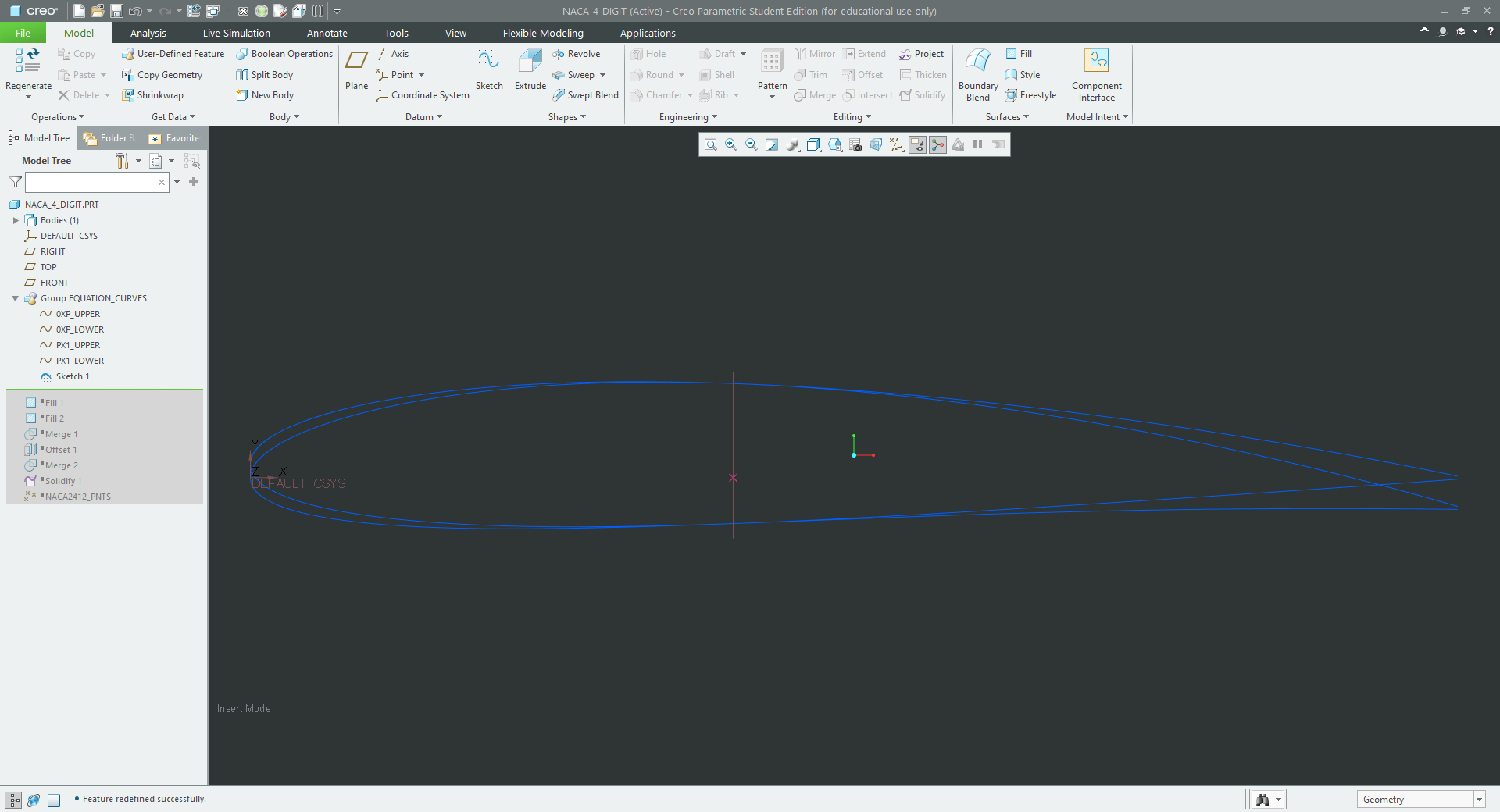figure 5 - Final curve from equations

The surface skteches will now be made. I tried creating just a single sketch but at point 'p' the software was having issues stating that "sketch has incomplete sections", splitting it into two surfaces worked. I could then merge the surfaces together. 

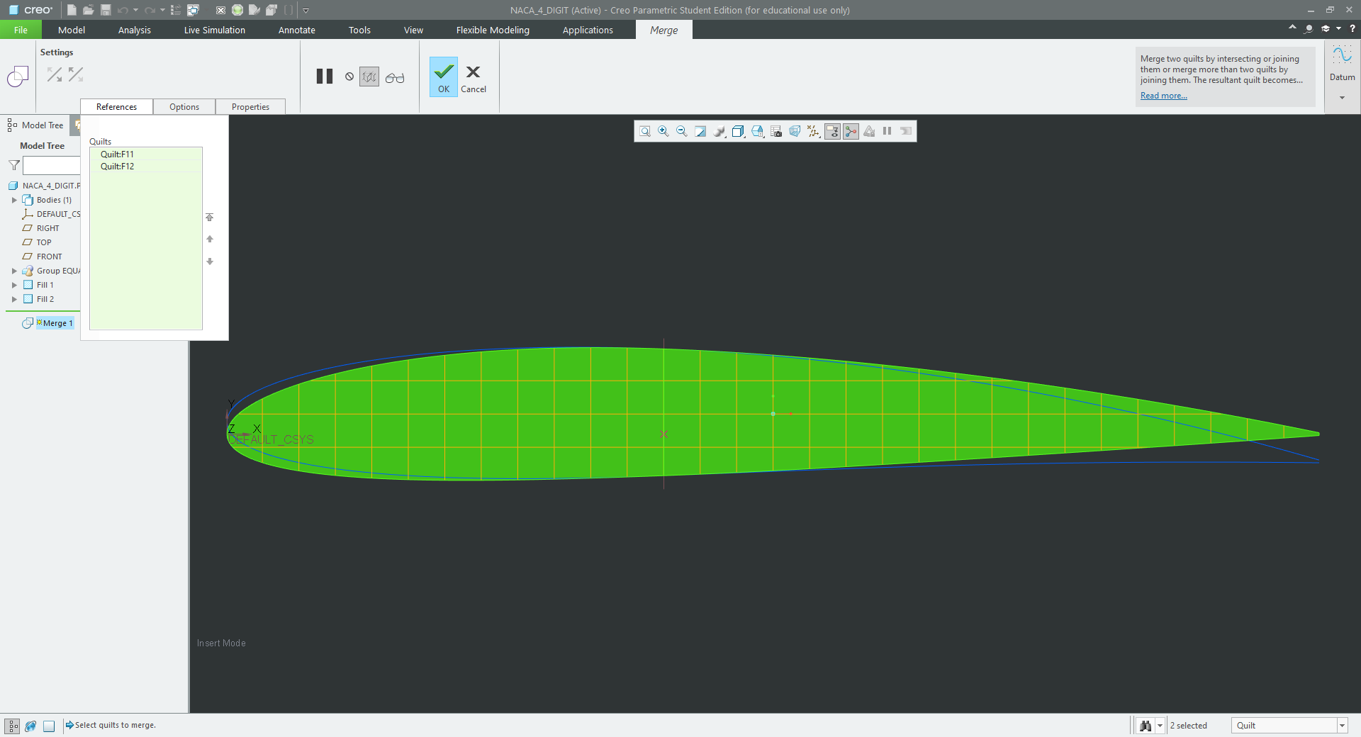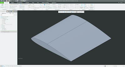
figure 6 - merge of the two surfaces to create the aerofoil profile

Thickening the profile surface to the desired wingspan, in this case 1m will then create a solid model.

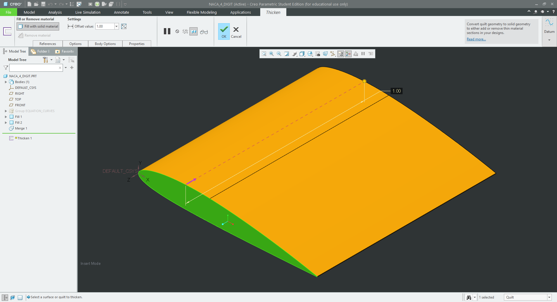figure 7 - Profile thickened and solidified

Completed Aerofoil

The geomtry is complete and the parameters can be modified to change the profile. Below will illustrate a few examples of different aerofoil profiles that can be quickly modified. For inverted aerofoils the equaitions can be multipled by -1.

Advantages/Disadvantages

Naturally not every choice is perfect for all scenarios. The key advantage of modelling with this method is the flexibility in changing the aerofoil geometry and the time saved from modelling different profiles of the same equation.

It is also useful if you know that your aerofoil is one continuos chord length along the wingspan as the chord length can't be easily modified. Within Creo the only way I can change the chord length (that I know of) is if I scale the model, this could potentially end up resulting in a messy model if multiple chord lengths were required along the span.

Formula 1 front wing would be a great example as some of the flaps have drastically varying chord lengths along the span.

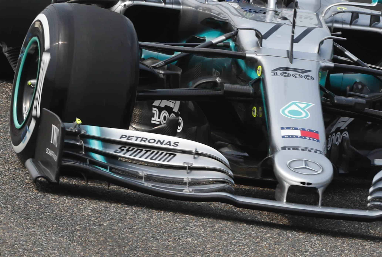https://maxf1.net/wp-content/uploads/2019/04/Mercedes-F1-W10-new-front-wing-endplate-Chinese-GP-F1-2019-Photo-Daimler-Edited-by-MAXF1net.jpg

feel free to download the model and have a look yourself (requires creo 7.0+)